Classical methods of border detection
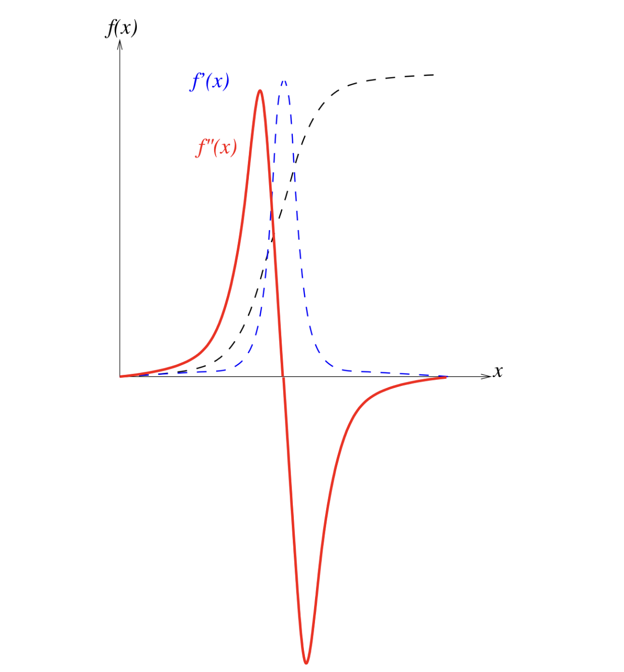
We try to use the local variations of the image to find borders: the 1st and 2nd derivatives.
Since we are looking for discontinuities in the image, we need to find the points where the derivative is maximum. This is equivalent of looking for places where the second derivative is zero.

For any image $I$, we have:
$$ \begin{align*} \nabla I &= \begin{pmatrix} I_x \\ I_y \end{pmatrix} \\ | \nabla I | &= \sqrt{I_x^2 + I_y^2} \\ \theta &= \arctan{\left(\frac{I_y}{I_x}\right)} \end{align*} $$Naive approach
The simplest approximation is:
$$ \begin{align*} I_x(i, j) &= I(i + 1, j) - I(i, j) \\ I_y(i, j) &= I(i, j + 1) - I(i, j) \\ \end{align*} $$We can, then, define a threshold $\lambda$ and extract the points where $| \nabla I | > \lambda$. Problem: very sensitive to noise. Solution: pre-filter with low-pass filter.
Sobel filtering
Sobel does just that: it uses a low-passing filter, followed to the naive approximation of the derivative:
$$ S_x(I) = \begin{pmatrix} 1 & 0 & -1 \\ 2 & 0 & -2 \\ 1 & 0 & -1 \end{pmatrix} \ast I \qquad \qquad S_y(I) = \begin{pmatrix} 1 & 2 & 1 \\ 0 & 0 & 0 \\ -1 & -2 & -1 \end{pmatrix} \ast I $$Zero-crossing Laplacian
We can also use the second derivative to find edges. We are looking for the places where
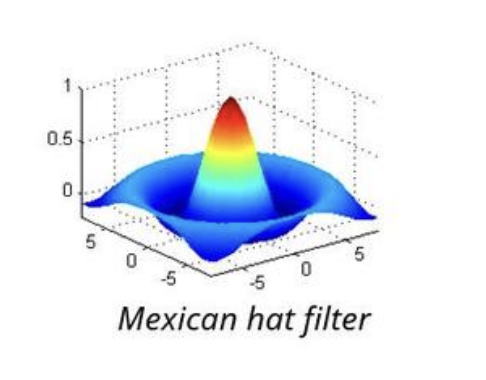
$$ \begin{align*} \Delta (G_\sigma \ast I) &= 0 \\ \implies (\Delta G_\sigma) \ast I &= 0 \end{align*} $$where $G_\sigma$ is the Gaussian filter. Using the equation above, it is easy to see that we can pre-compute $\Delta G_\sigma$ and not need to derivate the image. After filtering the points where $(\Delta G_\sigma) \ast I = 0$, we select those where $| \nabla I | \geq \sigma_1$.
We are able to approximate $\Delta G_\sigma$ with a difference of Gaussians:
$$ \Delta G_\sigma = \frac{1}{\sigma} \frac{\partial G_\sigma}{\partial \sigma} $$
A good algorithm that implements this idea is Canny’s algorithm.
Canny’s algorithm
Noise reduction:
$$ I_\sigma = G_\sigma \ast I $$Local maxima in gradient’s direction: The algorithm filters from $| \nabla I_\sigma |$ the pixels that are local maxima in the direction of the gradient.
Double Thresholding: Here, we apply two thresholds: $\sigma_1 < \sigma_2$ (weak and strong egdes).
$$ \begin{align*} E_1 &= \{x \colon |\nabla I_\sigma(x)| \geq \sigma_1\} \\ E_2 &= \{x \colon |\nabla I_\sigma(x)| \geq \sigma_2\} \end{align*} $$Hysterisis: All strong edges (pixels from $E_2$) are retained. A pixel from $E_1$ is considered only if it is connected to a pixel in $E_2$.
Global methods of region extraction
Since these methods are global, they do not use spacial information.
Binary segmentation

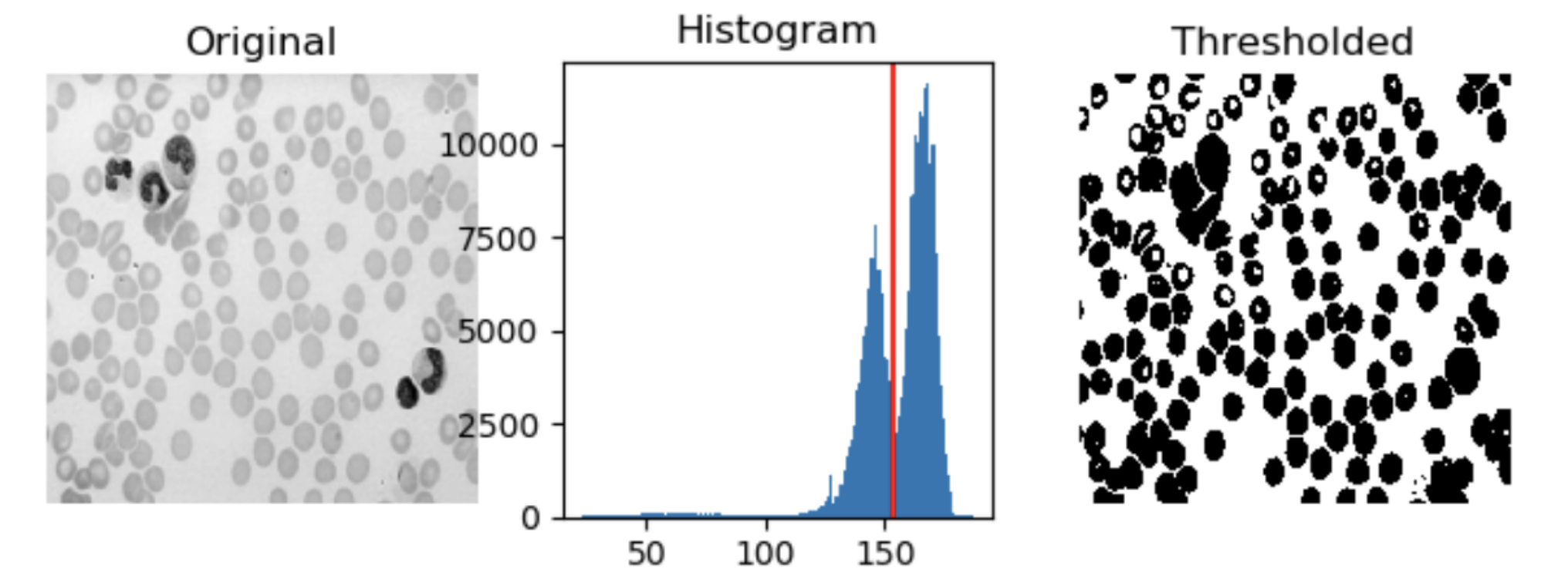
Otsu’s method
In this method, we want to minimize the intra-class variation and maximize the inter-class variation. To this end, let $T$ be the threshold applies and $H$ be the cumulative histogram of the image. Suppose $\mu_0(T)$ and $\sigma_0^2(T)$ are the mean and variance of the class 0 and $\mu_1(T)$ and $\sigma_1^2(T)$ the mean and variance of the class 1. Then, we can define the intra-class and inter-class variations as:
$$ \begin{align*} \sigma_w^2(T) &= H(T) \sigma_0^2(T) + (1 - H(T)) \sigma_1^2(T) \\ \sigma_b^2(T) &= \sigma^2 - \sigma_w^2(T) \end{align*} $$where $\sigma^2$ is the variation of all pixel values.
Clustering in many dimensions
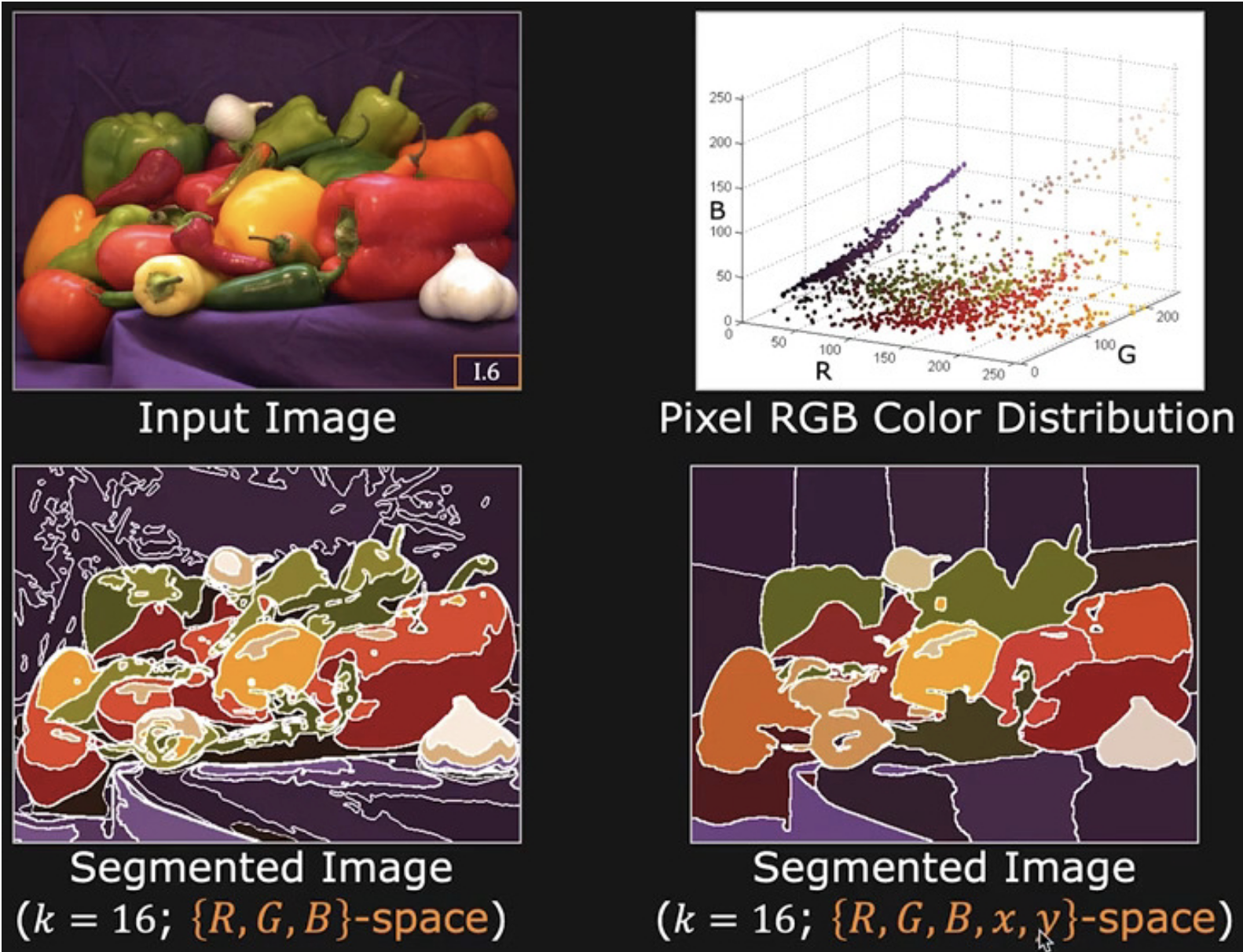
When we deal with colored images, we might express the histogram in 3 dimensions. Then, we can apply the K-means clustering algorithm to segment the image.
If we want to also take into account the spatial information, we can do the same thing, but with 5 dimensions.
