There are inherit defects when an image is captured.
Noise
The noise is an error of measurement in each pixel. There are essentially 2 sources:
- Read noise (uniform);
- Photonic noise (depends on the luminosity): each photon has a probability $p$ to be measured ($p < 1$ to read only the color we want) in a Poisson distribution, then, $\mathbb{E}[Y] = N p (1 - p)$ and $\mathrm{Var}(Y) = N p (1 - p)$.
The relative photonic noise is, however,
$$ \frac{\sqrt{\mathrm{Var}(Y)}}{\mathbb{E}[Y]} = \frac{1}{\sqrt{N p (1 - p)}} $$so, the darker the place, the greater the relative noise.

Blur
The blur can come from a variety of sources:
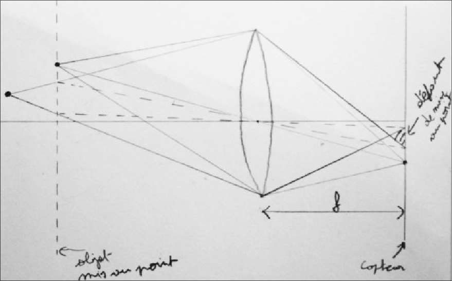
- Optic: Good camera adjustment (less than 1 pixel of blur from field depth);

- Atmospheric turbulence: Gaussian model;
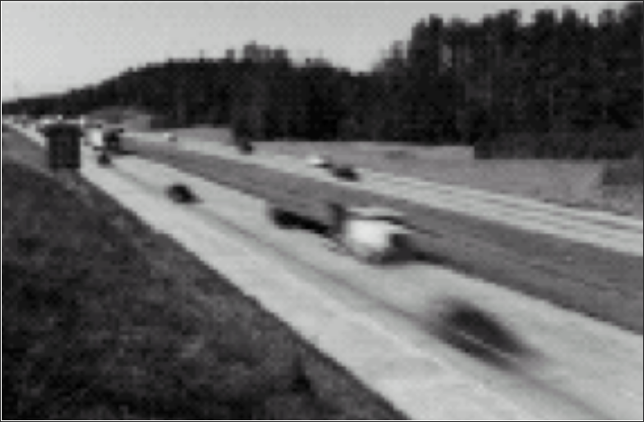
- Movement;

- Diffraction: $\theta \propto \frac{\lambda}{D}$.

Bad sampling
The optic capacity is limited by the diffraction.

Defects model
$$ g = f \ast K + b $$where:
- $f$ is the perfect image;
- $g$ is the observation;
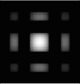
- $K$ kernel of blur;
- $b$ noise (we suppose it is uniform and independent of the signal).
We will also suppose that the discretization is without loss and that the image is periodic. Then, we can rewrite as
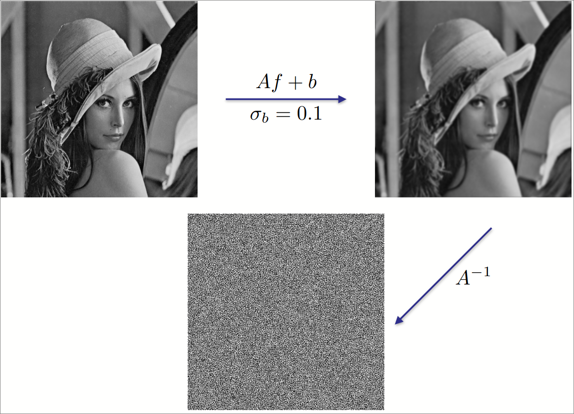
$$ g = A f + b $$where $A$ is the convolution matrix $N^2 \times N^2$ and $f$, $g$ and $b$ are matrices $N \times N$.
We cannot, though, just try to invert $A$ and compute $A^{-1}g$:

Wiener restoration
1-dimensional case
Before going to the general solution, we will consider the restoration of a single pixel, i.e., in 1 dimension. In this case, we have the following model:
$$ Y = \alpha X + B $$where $X$ is the “real” pixel with mean $0$ and variance $\sigma_s^2$, $Y$ is the value observed and $B$ is a random Gaussian noise with variance $\sigma_b^2$.
Our goal is to find $\tilde{X}$ that is an approximation of $X$ such that
$$ \tilde{X} = \beta Y $$while keeping the lowest error possible. The error is given by
$$ \mathbb{E}[{\vert \tilde{X} - X \vert}^2] $$The solution for this 1-dimensional case is
$$ \beta = \frac{\bar{\alpha}}{{\vert \alpha \vert}^2 + \frac{\sigma_b^2}{\sigma_s^2}} $$The idea is that when the noise is low compared to the signal (low $\frac{\sigma_b^2}{\sigma_s^2}$), we can just use the inverse of $\alpha$. If, however, the noise is high compared to the signal (high $\frac{\sigma_b^2}{\sigma_s^2}$), we just assign $\beta = 0$ because there is no meaningful information to be extracted from the signal.
General case
The general case of Wiener restoration is given by the following model:
$$ Y = A X + B $$where $X$ and $B$ are Gaussian random vectors. Now, we want to find $\tilde{X} = D Y$, where $D$ is a linear operator, while minimizing $\mathbb{E}[{\vert \tilde{X} - X \vert}^2]$. The solution is given by
$$ D = (A^\top A + \sigma_b^2 C^{-1}) A^\top. $$where $C$ is the covariance matrix of $X$ ($C = \mathbb{E}[X X^\top]$)
Still, computing $D$ is extremely expensive, since the covariance matrix $C$ is very large (quadratic on the number of pixels).
To fix this issue, we can apply additional hypothesis and try to restore the image in the Fourier domain. Then, we need to define a power spectral density $\sigma_s^2(\omega)$ and use the following formula:
$$ \hat{\tilde{f}}(\omega) = \frac{\bar{\hat{K}}(\omega)}{{\vert \hat{K}(\omega) \vert}^2 + \frac{\sigma_b^2}{\sigma_s^2(\omega)}} \hat{g}(\omega) $$The hats on top of the functions in the formula just indicate that we are in the Fourier domain of their respective functions. Here, $K$ is the convolution kernel (so we suppose that $Af$ can be represented as $K \ast f$).
So the final idea is to do a Fourier Transform on the observed image and, then apply the equation above to all frequencies $\omega$. After that, we just do the Inverse Fourier Transform to get the restored image.
There are many ways to choose $\sigma_s^2(\omega)$. The most commons are:
- $\sigma_s^2(\omega) = {\vert \hat{g}(\omega) \vert}^2$;
- $\sigma_s^2(\omega) = \omega^{-\beta}$, where $\beta$ is near $2$;
Energy minimization
Another way to model the restoration of images is to make the restored image minimize the following energy:
$$ E(\tilde{f}) = \underbrace{{\Vert A \tilde{f} - g \Vert}^2}_{\text{similarity with data}} + \underbrace{\lambda \int {\Vert \nabla \tilde{f} \Vert}^2}_{\text{regularity}} $$The solution to this minimization problem is
$$ \hat{\tilde{f}}(\omega) = \frac{\bar{\hat{K}}(\omega)}{{\vert \hat{K}(\omega) \vert}^2 + \lambda \omega^2 \sigma_b^2} \hat{g}(\omega). $$What is interesting is that this is equivalent to applying the Wiener restoration with a power spectral density $\sigma_s^2(\omega) = \omega^{-2}$. This last model is, nonetheless, weak and simplifies way to much the blur model.