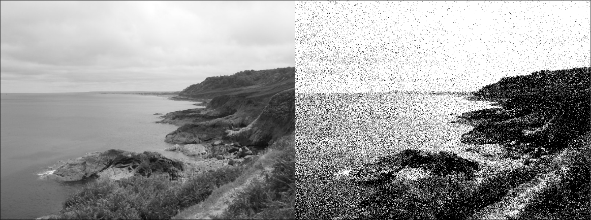
The perception of an image’s content changes little when an increasing function is applied to it. However, if the function is non-increasing, then the perception of the content changes completely. We are sensible to local rather than global changes of contrast.
From now on, we are denoting $u \colon \Omega \to \mathbb{R}$ our image, where $\vert \Omega \vert = M \times N$ is a discrete rectangular grid. Also, we are assuming that $u$ takes discrete values $y_0 < \dots < y_{n - 1}$ (usually $0$ to $255$).
Histograms
We can define the histogram $h_u$ of an image $u$ as follows:
$$ h_u = \sum_{i = 0}^{n - 1} \delta_{y_i} \underbrace{\frac{\vert \{ \mathbf{x} \in \Omega \mid u(\mathbf{x}) = y_i \} \vert}{\vert \Omega \vert}}_{h_i} $$where $\delta_{y_i}(y)$ is the indicator function $1$ if $y = y_i$ and $0$ otherwise.
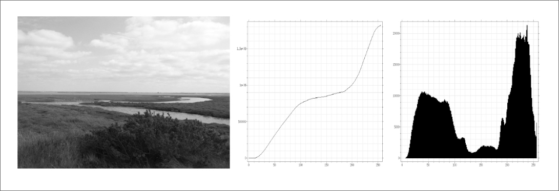
The histogram characterizes de distribution of gray levels in an image.
Let $u$ be a discrete image defined on a grid $\Omega$. The cumulative histogram of $u$ is the function $H_u$ defined as follows:
$$ H_u(\lambda) = \frac{\vert \{ \mathbf{x} \in \Omega \mid u(\mathbf{x}) \leq \lambda \} \vert}{\vert \Omega \vert} $$If $g$ is a strictly increasing contrast change, then
$$ H_{g(u)}(g(y_i)) = H_u(y_i) \qquad \forall i $$Classical contrast changes
Luminosity & contrast
$$ u \mapsto ku + C $$where $k$ is the contrast and $C$, the luminosity. If $k$ and $C$ are chosen so that the new image uses all the $y_i$, we call this contrast stretching.

Seuillage
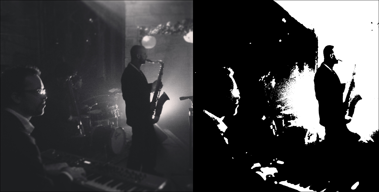
$$ u \mapsto \mathbb{1}(u > \lambda) $$Image turns binary.
Gamma transformation
$$ u \mapsto u^\gamma $$Older cameras would capture images in a non-linear form. The gamma transformation was then used to “cancel” the non-linear aspect of the image (usually $\gamma = 2.5$).

Histogram equalization
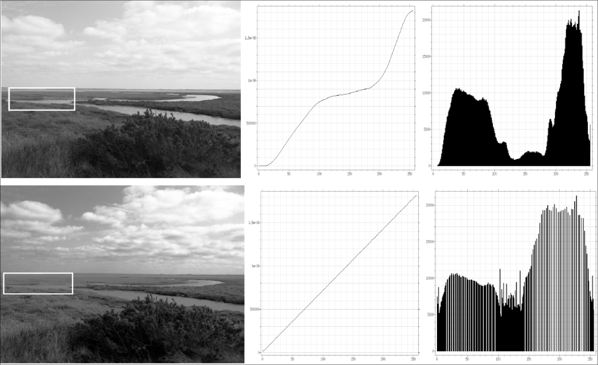
We call this operation “equalization” because the cumulative histogram of the result, $H_{g(u)}$ approximates the identity function. More precisely,
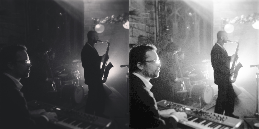
However, the equalization has a big flaw: regions with great contrast differences in the original image might have little contrast changes in the final image. We can observe this phenomenon in the following image:
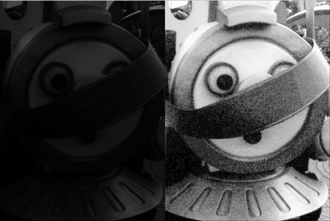
Furthermore, the equalization can increase the quantification noise.
Histogram specification
Now, instead of $H_{g(u)} \approx \mathrm{Id}$, we want $H_{g(u)}(\lambda) \approx F$, given an arbitrary strictly increasing function $F$. To this end, we can set $g \equiv F^{-1} \circ H_u$.
Then, just like the histogram equalization, we will have $H_{F^{-1} \circ H_u \circ u}(\lambda) \leq F(\lambda)$ with equality when $\lambda = (F^{-1} \circ H_u)(y_i)$.

We can go further and try to give to $u$ the same histogram as another image $v$. To do so, we can simply set $F \equiv H_v$ and use histogram specification.
However, we cannot be sure that $H_v^{-1}$ exists! To solve this problem, we can define a pseudo-inverse of $H_v$ as follows:
In simpler terms, this means that $H_v^{-1}$ will be constant by parts and for every point $\mathbf{x} \in \Omega$, we have $(H_v^{-1} \circ H_v)(v(\mathbf{x})) = v(\mathbf{x})$.
Quantification
Usually, the cameras are able to capture images with more than $8$ bits. So, the idea is to “fit” the captured image into 8 bits. To do so, we have a quantification operator.
We do so by slicing the values captured by the camera in intervals $[t_i, t_{i + 1}]$. Then, we assign $q_i$ (8 bits) to every value in $[t_i, t_{i + 1}]$.
There are many ways to choose $t_i$.
Uniform: $t_i = \frac{256 i}{p}$ and $q_i = \frac{t_i + t_{i + 1}}{2}$.
Following histogram: $t_i = \min{\{ \lambda \mid H_u(\lambda) \geq \frac{i}{p} \}}$ and $q_i$ are the means (or barycentre) of the intervals. This makes the histogram equalized before uniform quantification.
Lloyd-Max: Minimizes de squared error.
Dithering
We want to binarize de image in a clever way. To do so, we can add a noise to the image and, then, binarize it. The noise makes it more likely to get black in the regions with more blackish pixels. This results in a better binarization.
$$ P(x + N > 128) = P(N > 128 - x) = \int_{128 - x}^{\infty} f(t) dt $$