The pinhole model
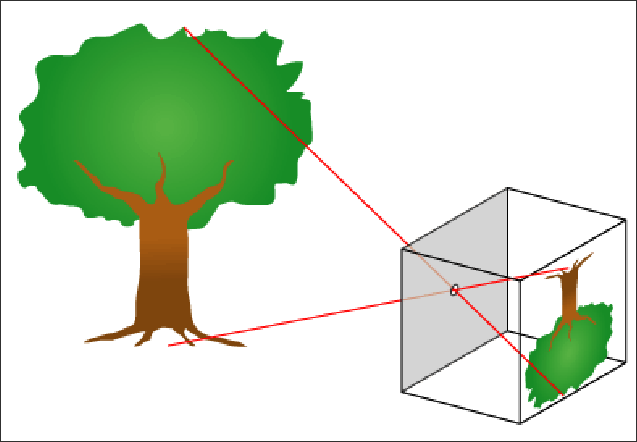
The first very simple way to acquire images is with the pinhole model. Here, part of the light coming from the object passes through a small aperture $O$ and is projected onto the focal plane. We do this so that each point of the object is represented by a ray. Otherwise, the image would not be formed.
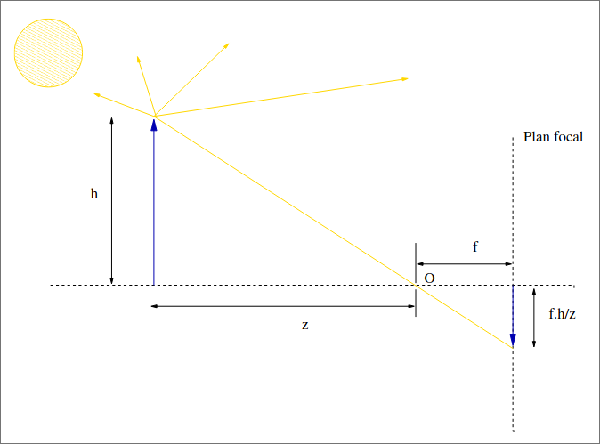
The distance $f$ is called the focal length. Let’s suppose we have the following model to describe the pinhole:
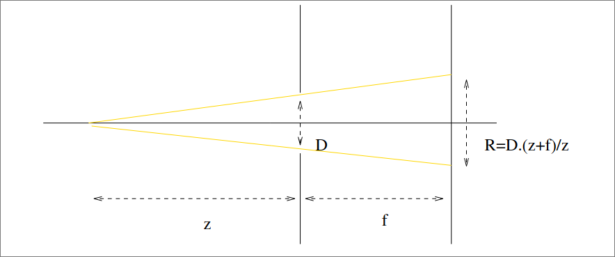
Since the aperture $O$ is finite, the rays produce blur. This effect can be modelled by
$$ g_z \ast S $$where $S$ would be the “real” image and $g_z$ is the indicator function of a disk of radius $\frac{(z + f) D}{z}$.
Using lenses
For a sharper image, we can add a lens. It behaves as shown in the following image.
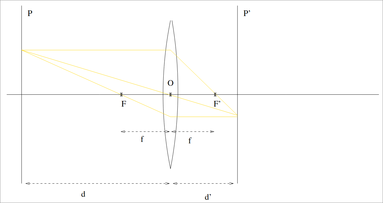
To remember:
- Horizontal rays converge at the focal point;
- Rays passing through the origin $O$ do not change;
- Rays passing through a focal point exit horizontally.
The focal distance $f$ can be calculated using Descartes’ Relation.
$$ \frac{1}{d} + \frac{1}{d^\prime} = \frac{1}{f} $$Depth of field
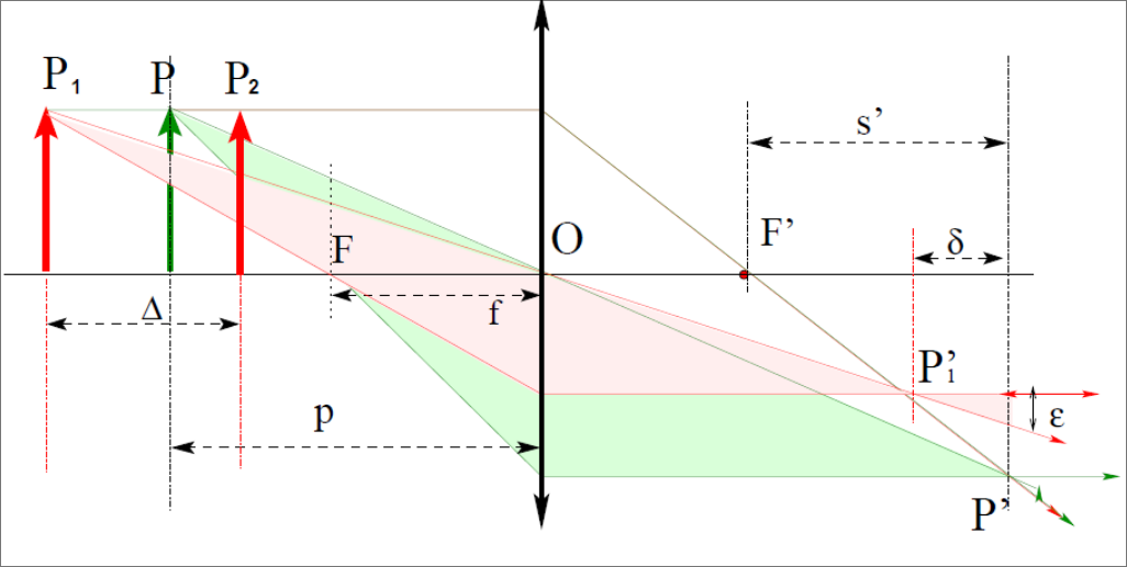
Depth of field is the distance separating the sharp object closest to the camera from the farthest sharp object.
$$ \Delta \approx \frac{2 \varepsilon p^2}{D f} $$where $p$ is the object distance.
- e.g. $f / 4$ means $N = 4$.
When $N$ increases (at constant $f$):
- $\Delta$ increases;
- Diffraction defects increase;
- Vignetting defects (darker image near bords) increase;
Sampling
Now the aim is to transform the photons in the image into something electrical that can be digitized.
$$ \left( f \colon \mathbb{R}^2 \mapsto \mathbb{R} \right) \rightarrow (\{f(k)\}_{k \in \Omega}). $$Photon counting can be formalized mathematically by convolution with $g_{text{capt}}$, which is the sensor’s indicator function.
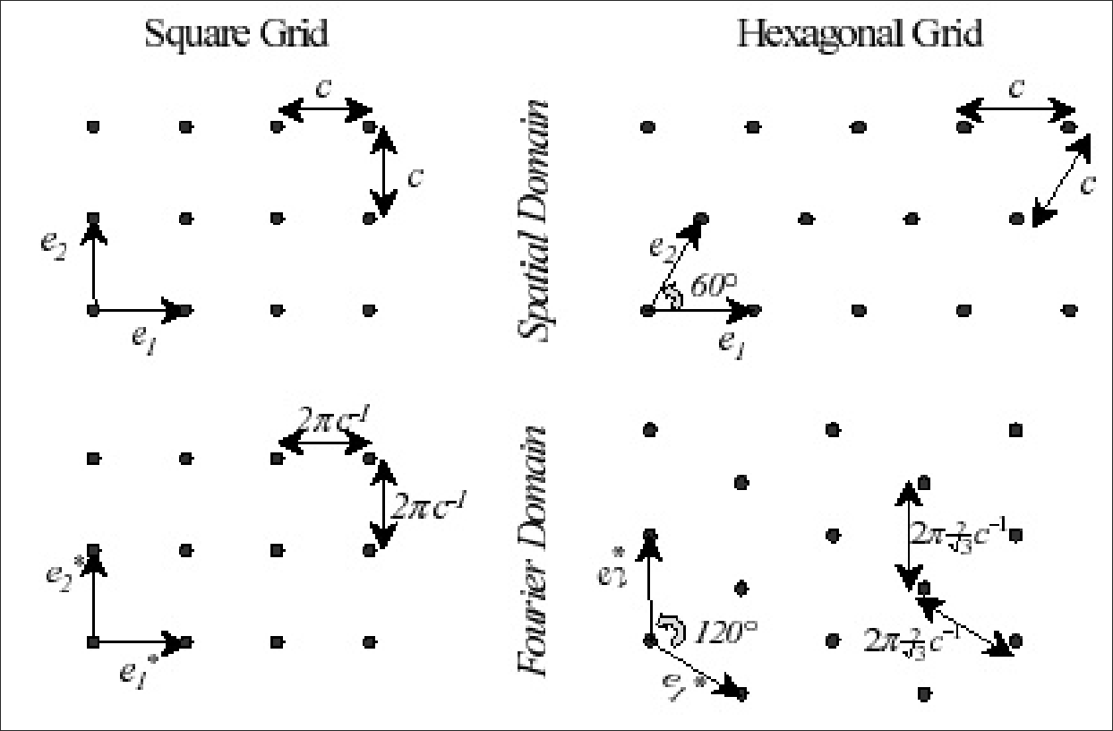
$$ I_{i, j} = (I \ast g_{\text{capt}})(i, j) $$The following image shows an example of a sensor grid.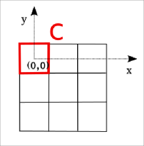
The sampling of a function $f$ at a point $\mathbf{x}$ is modeled by
$$ f \cdot \delta_{\mathbf{x}} $$So, to model image acquisition, we’ll use Dirac’s comb, $\Pi_\Gamma$, which is defined shortly.
$$ \Pi_\Gamma = \sum_{\gamma \in \Gamma} \delta_\gamma $$where $\Gamma$ is the set of positions where the detectors are placed (e.g. $\Gamma \subset \mathbb{N}^2$).
We can also place the detectors in a hexagonal array. This can sometimes be advantageous.
