Decision Trees & Random Forests

Classification models

We are interested in classifying a data set among many classes. Each point in the data set has many attributes. Those can be either discrete or continuous, but the classes can only be discrete. If a continuous class is required, then we should use a regression model. It is also worth noting that the classes have no order relation (we cannot say that class 5 is greater than class 2).

Underfitting & overfitting

Underfitting: the model is too simple to fit the data. It performs poorly both in the training and test sets. Overfitting: the model is too complex to fit the data. It performs poorly in the test set, but has a great accuracy in the train set.

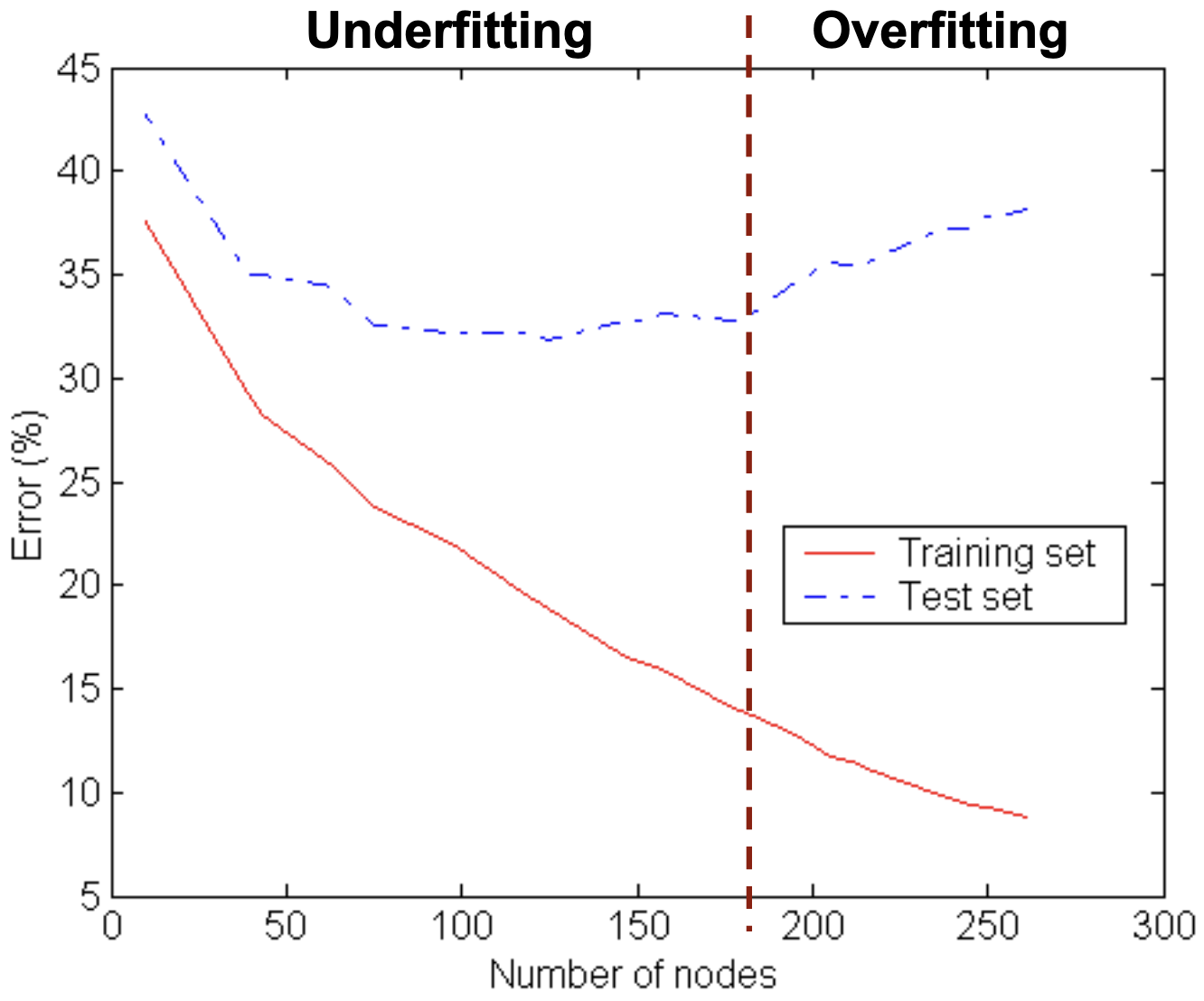
Overfitting can be caused by many things:

• Noise in training data;
• Insufficient data;

Model evaluation

$$ \text{Accuracy} = \frac{TP + TN}{TP + FP + TN + FN} $$

The accuracy can be misleading in some settings. E.g., if the model always predicts the default class, then the accuracy approaches $100\%$ if most records are of the default class.

$$ \begin{align*} \text{Precision} = p &= \frac{TP}{TP + FP} \\ \text{Recall} = r &= \frac{TP}{TP + FN} \end{align*} $$

Usually, $p$ and $r$ balance each other out. If we predict everything as “Positive”, $r$ gets really high, but $p$ gets really low. The inverse happens when we predict “Positive” when we are extremely sure. To consider both, we can use the F1-score.

$$ \text{F1-score} = \frac{2 p r}{p + r} $$

Decision trees

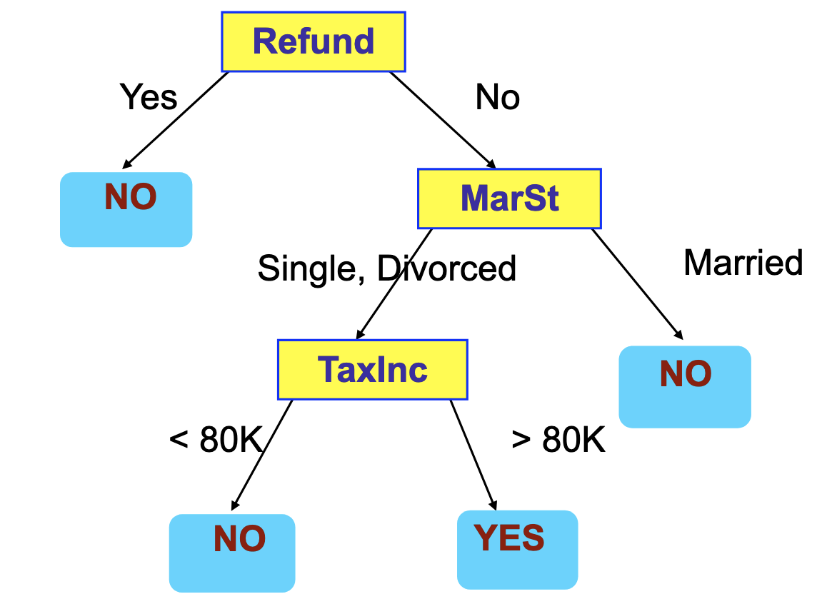
We model the classification problem using a tree. Each internal node represents a split in the data set based on an attribute (splitting attributes). The leaves represent the classes.

Note that multiple trees may fit the same data set. The following figure shows an example of a decision tree that identifies tax fraud.

There are many ways to fit a tree to the data set. We are going to focus on Hunt’s algorithm.

Let $D_t$ be the set of training records that reach a node $t$. The outline of the algorithm is:

• If all elements in $D_t$ are of the same class, then $t$ becomes a leaf of this class;
• If $D_t = \emptyset$, then $t$ becomes a leaf of the default class;
• If $D_t$ contains elements from multiple classes, use an attribute test to split the data into smaller subsets.

Then, we recursively apply these steps. In the end, we will have a tree fitted to our training data set. So, how can we split the data? A greedy strategy will be used. The division is made to optimize a criterion.

How to specify the test condition?

Depends on the attribute type:

• Ordinal;
• Categorical;
• Continuous.

Depends on the number of splits:

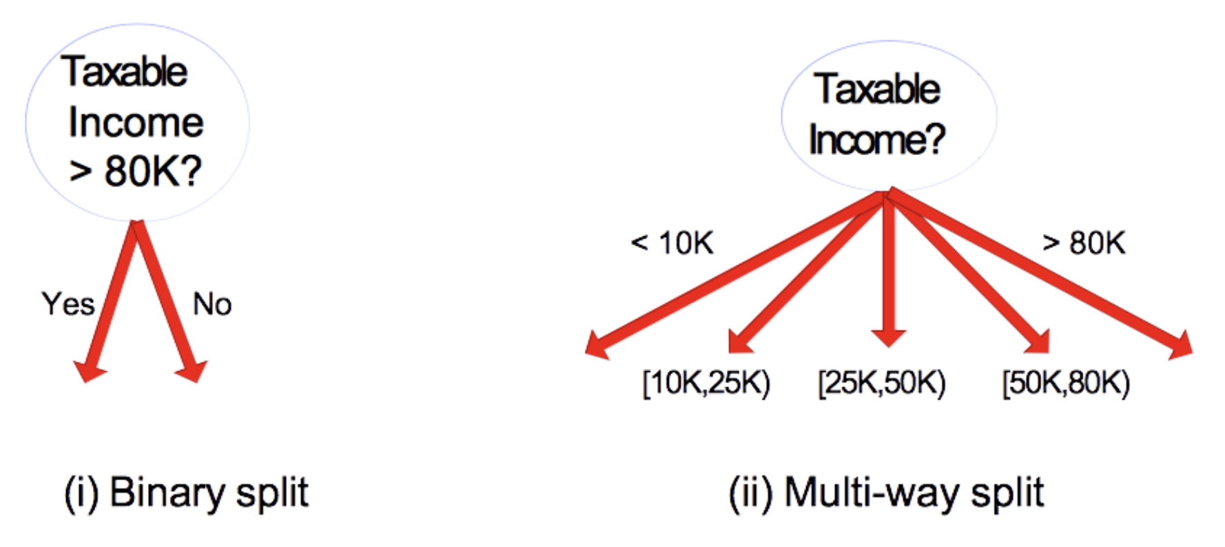
• Binary split;
• Multi-way split.

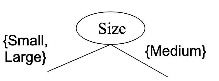
Note that when splitting ordinal attributes, we still have to respect the intrinsic ordering.

When dealing with continuous attributes, we have two options:

1. Discretization of the attribute: either as a pre-processing or dynamically (e.g. K-Means clustering), or
2. Binary split: Find the best split $(A < v)$ or $(A \geq v)$.

How to determine the best split?

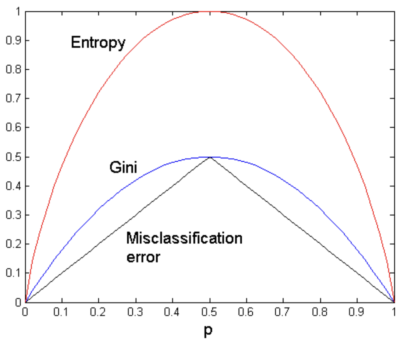
Here, a greedy strategy is used to separate well the data. Our goal is to have a very homogeneous split. There are 3 greedy functions we can maximize:

• Gini index;
• Entropy;
• MisClassification error.

Gini index

Let $t$ be an internal node in the tree, and $C$ be the set of classes.

$$ \mathrm{GINI}(t) = 1 - \sum_{c \in C} [\mathbb{P}(c \mid t)]^2 $$

where $\mathbb{P}(c \mid t)$ is the probability of class $c$ in node $t$.

It is easy to see that $\mathrm{GINI}(t)$ reaches its minimum when all records in $D_t$ belong to the same class. Then, $\mathrm{GINI}(t) = 1 - 1^2 = 0$. This function reaches its maximum when the records in $D_t$ are equally distributed among all classes. In this case, if each class has $n_c$ records in node $t$,

$$ \begin{align*} GINI(t) &= 1 - \sum_{c \in C} \left(\frac{n_c}{|D_t|}\right)^2 \\ &= 1 - \sum_{c \in C} \left(\frac{n_c}{n_c |C|}\right)^2 \\ &= 1 - \sum_{c \in C} \frac{1}{|C|^2} \\ &= 1 - |C| \frac{1}{|C|^2} \\ &= 1 - \frac{1}{|C|} \end{align*} $$

We are interested in minimizing the Gini index.

Suppose we split node $t$ into child nodes. We will call $I$ the set of child nodes. Let $n_i$ be the number of records in node $i \in I$ and let $n = |D_t|$. Then, we can define the Gini of the split as follows:

$$ \mathrm{GINI}_\text{split}(t) = \sum_{i \in I} \frac{n_i}{n} \mathrm{GINI}(i) $$

We can also define the Gini gain:

$$ \mathrm{GiniGain}(t) = \mathrm{GINI}(t) - \mathrm{GINI}_\text{split}(t) $$

With continuous attributes, we have to find a value $v$ such that the binary split has minimum Gini. To find $v$ efficiently, we can order the values of this attribute in the data set. Then, compute the Gini incrementally. This ends up being a $\mathcal{O}(n \log{n})$ algorithm.

Entropy

We are also able to use the entropy as a criterion for our greedy algorithm.

$$ H(t) = - \sum_{c \in C} \mathbb{P}(c \mid t) \log \mathbb{P}(c \mid t) $$

Its minimum value is reached when all records in $D_t$ belong to the same class and it is $H(t) = 0$. The maximum corresponding to an even distribution and is $H(t) = \log{|C|}$.

Just like with the Gini index, we can define the entropy of the split as the entropy gain:

$$ H_\text{gain}(t) = H(t) - \sum_{i \in I} \frac{n_i}{n} H(i) $$

Disadvantage: entropy tends to prefers splits that result in large number of partitions. Each of them is very pure, but very small.

We can solve this issue by considering the Gain ratio:

$$ \begin{align*} H_\text{split}(t) &= - \sum_{i \in I} \frac{n_i}{n} \log{\left( \frac{n_i}{n} \right)} \\ \mathrm{GainRatio}_\text{split}(t) &= \frac{H_\text{gain}(t)}{H_\text{split}(t)} \end{align*} $$

This way, a large number of partitions is penalized.

Classification error

$$ \mathrm{Error}(t) = 1 - \max_{c \in C} \mathbb{P}(c \mid t) $$

Then, $\min{(\mathrm{Error}(t))} = 0$ and $\max{(\mathrm{Error}(t))} = 1 - \frac{1}{|C|}$.

When to stop splitting?

There are many stopping criteria that can be used:

• Stop when all $D_t$ belong to the same class;
• Stop when all records have very similar attribute values;
• Early termination.

Quantify error

The generalization error is defined as follows:

$$ E_\text{gen} = E_\text{train} + \alpha * L $$

where $E_\text{train}$ is the number of errors in the training set, $L$ is the number of leaves in the tree and $\alpha$ is usually $0.5$.

Pruning

After a tree is fitted, it can be pruned to improve the generalization error. To this end, we check for each subtree if it would be best to replace it by a single node. This is done by comparing the generalization error of the new tree with the old one.

We usually compute this algorithm in a bottom-up manner.

Conclusion

Advantages of using decision trees:

• Inexpensive to construct;
• Very fast at classifying new data;
• For small trees, easy to interpret;
• Accuracy comparable to other methods.

Issues of using decision trees:

• Data fragmentation: Number of instances get smaller as you go down the tree. Then, data in leaves might be statistically irrelevant;
• Search strategy: Finding an optimal tree is NP-hard;
• Expressiveness: Does not model well continuous attributes;
• Tree replication: The same subtree may appear multiple times inside the decision tree.

Random forests

Here, the idea is to use many decision trees to decrease the variance of the model (i.e., making it more precise). Suppose we have $N$ records, each with $M$ features.

Parameters:

• $k$: number of trees;
• $t$: number of attribute (usually $\sqrt{M}$).

Then, we separate the data set into $k$ subsets. Each tree $T_i$ will be trained on a set $S_i$ of the data. $S_i$ contains $N$ records randomly samples (with replacement) from the original data set. This means that a record $x_j$ may appear more than once in $S_i$. We also select $t$ random features (without replacement, to avoid repeated attributes) from the training data.

Finally, we train each tree $T_i$ separately. To predict the class of a new data point $y$, we simply take the majority class among the predicted classes of the $k$ trees.