Clustering

Our goal in clustering is to group similar data points together. Each group will be called a cluster. Ideally, the intra-cluster distances are minimized and the inter-cluster distances are maximized.

Note that this is an unsupervised model, so the following cannot be considered as clustering:

• Supervised classification;
• Simple segmentation;
• Results of a query;
• Graph partitioning.

There are two types of clustering:

• Partitional clustering: divide data into non-overlapping subsets & each data is in exactly one subset;
• Hierarchical clustering: A set of nested clusters organized as a hierarchical tree.

Types of clusters

• Well-separated cluster: any point in the cluster is closer to every other point in the cluster than to any point not in the cluster;
• Center-based cluster: An object in the cluster is closer to its center than to the center of other clusters. The center is usually the centroid or medoid (most representative point);
• Contiguous cluster: a point in the cluster is closer to one or more other points in the cluster than to any point not in the cluster;
• Density-based cluster: A cluster is a dense region of points, which is separated by low-density regions, from other regions of high density;
• Conceptual cluster: Clusters that share some common property or represent a particular concept.

K-means clustering

Input: A set $S$ of points in the euclidean space and an integer $k > 0$.
Output: A parititonal clustering of $S$.

1. Select $k$ points from $S$ to be the initial centroids.
2. Repeat until the centroids do not change:
   • Form $k$ clusters by assigning each point in $S$ to the closest centroid.
   • For each cluster, recompute the centroids.

Here, the initial centroids are chosen at random.

Evaluation

The most common way to evaluate a K-means clustering is to compute the Sum of Squared Errors (SSE):

$$ \text{SSE} = \sum_{i = 1}^{k} \sum_{x \in C_i} \mathrm{dist}^2(m_i, x) $$

where $m_i$ is the centroid of cluster $C_i$ and $dist$ is the Euclidean distance between two points. The SSE can be seen as the sum of the variances of the clusters.

Usually, the lower the $k$, the higher the SSE. However, good clustering with small $k$ has lower SSE than a poor clustering with large $k$.

Pre-processing:

• Normalize the data;
• Eliminate outliers.

Post-processing:

• Eliminate small clusters that may represent outliers;
• Split clusters with high SSE;
• Merge clusters that are close and have low SSE.

Correctness

Empty cluster problem

The problem will be solved in 1 dimension. Let $S = \{1, 9, 10, 18, 19, 20.1\}$, $k = 3$, and the initial centroids be $m_1 = 1, m_2 = 18, m_3 = 20.1$.

First iteration:

• $C_1 = \{1, 9\}$ and $m_1 = 5$.
• $C_2 = \{10, 18, 19\}$ and $m_2 \approx 15.7 $.
• $C_3 = \{20.1\}$ and $m_3 = 20.1$.

Second iteration:

• $C_1 = \{1, 9, 10\}$ and $m_1 \approx 6.7 $.
• $C_2 = \{\}$.
• $C_3 = \{18, 19, 20.1\}$ and $m_3 \approx 19 $.

There are several solutions to the problem of empty clusters:

• Pick the points that contribute most to the SSE and assign them to the empty cluster;
• Pick the points from the cluster with highest SSE;

If there are multiple empty clusters, we can repeat these steps multiple times. A more robust solution is to update the clusters incrementally. This always works but is more expensive. We will show that this is the case.

Proof: Suppose a cluster $C$ would be empty in the next iteration of the usual algorithm. It is easy to see that $|C| > 1$ (otherwise, it would never be empty in the next iteration). By incrementally updating $C$ to $C^\prime$, we have $|C^\prime| = |C| - 1 \geq 1$. If $|C^\prime| = 1$, then $C^\prime$ will never be empty. Otherwise, $|C^\prime| > 1 > 0$, so it is not empty as well.

Limitations

K-means has problems when clusters are of different:

• Sizes;
• Densities;
• Non-globular shapes.

K-means also has problems when the data has outliers.

K-means++ clustering

In the K-means++ algorithm, the initialization of centroids is done in a clever way.

where

$$ \begin{align*} d(x, y) &= \Vert x - y \Vert \\ d(x, \mathcal{C}) &= \min_{c \in \mathcal{C}} d(x, c) \\ \Phi_X(\mathcal{C}) &= \sum_{x \in X} d^2(x, \mathcal{C}) \end{align*} $$

The denominator in the probability is always the same. The numerator, $d^2(x, \mathcal{C})$ is greater for points far from centroids. This means that points that are relatively far away from centroids are more likely to be selected. The consequence is a good clustering from the beginning.

Comparison with normal K-means

K-means	K-means++
No guarantees of quality of solution	$\mathcal{O}(\log{k})$-approximation on the quality of solution
Always terminates	Always terminates
Running time can be exponential, but OK in practice	Advantage noticible for large $k$

Hierarchical clustering

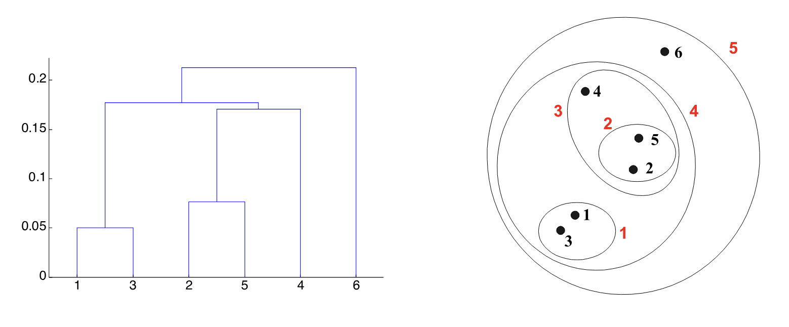
Hierarchical clustering produces a set of nested clusters organized as a hierarchical tree. This can be visualized as a dendrogram (a tree-like diagram that records merges and splits).

Advantages of this approach:

• We do not have to assume the number of clusters;
• It can correspond to meaningful taxonomies.

There are two main strategies to do hierarchical clustering:

• Start with one cluster per point and iteratively merge clusters that are close;
• Start with one cluster for all points and iteratively split clusters that are far.

The most popular algorithm goes as follows:

1. Let each data point be its own cluster;
2. Compute the distance matrix $n \times n$;
3. While there are multiple clusters:
   • Merge the two closest clusters;
   • Recompute the distance matrix;

Inter-cluster distance

There are many ways to define the distance between two clusters:

• The minimum distance between two points in the clusters;
• The maximum distance between two points in the clusters;
• The average of distances of every pairs of points in the clusters;
• The distance between the centroids.

Problems

The hierarchical clustering model has some limitations:

• Decisions to merge or split clusters cannot be undone;
• No error function is being directly minimized;
• High sensitivity to noise;
• Difficulty handling clusters of differing sizes and shapes.

Cluster validity

To compare various outputs and algorithms, we want to develop a way to quantify how good the clustering is.

If we want to measure how well a clustering classifies externally supplied class labels, we use entropy. If we want to measure the clustering structure without any external information, we use SSE. If we want to compare two clustering results, we can use either measure.

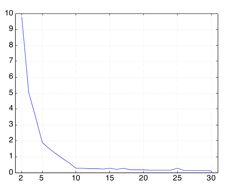
We usually use the SSE to estimate the best number of clusters through the elbow curve.

We can define the entropy and purity of a cluster as:

$$ \begin{align*} H_j &= - \sum_{i = 1}^k p_{ij} \log{p_{ij}} \\ P_j &= \max_{i} p_{ij} \end{align*} $$

Then, the entropy and purity of a clustering can be computed as:

$$ \begin{align*} H &= \sum_{j} \frac{m_j}{m} H_j \\ P &= \sum_{j} \frac{m_j}{m} P_j \end{align*} $$